We are going to steer away from the usual topics today because it’s getting to That Time of Year (holidays) and many people start fretting about their money situation, both leading up to the holidays and for the few weeks after the holidays when the bills come due. So, it seems like a good time to do an Excel tutorial on how to create a simple daily budget where you can transcribe your receipts and have Excel automatically total every category you set up and then total your spending and income.
Creating a budget is often daunting for people and many people would rather turn a blind eye to the whole thing, but taking control of your finances is extremely empowering.
And hey, learning some cool tricks in Excel is never a bad thing. So let’s go!
As a note, to make the most of this tutorial, you must have a tiny bit of prior knowledge of Excel. You should know how to select cells and type in cells.
Laying the Groundwork
Most of the work of this project is in the set up. There are a few things you’ll want to take notes on before we get going:
- Where you spend money (your monthly bills, groceries, clothing, entertainment, etc)
- What your income source(s) is/are
- Any savings you want to start up or maintain
You can scribble these things on a piece of paper if you like – the more prep we do before we actually start the sheet, the better.
Setting Up the Sheet
When we use Excel, the real trick to making it work properly is in the set-up. It’s tedious, but the more set-up we do now, the ‘smarter’ our sheet will be at the end.
So, here’s what we are going to start with:
- Open Excel and create a new blank Workbook
- Select Cells A1:I1 and then in the Home tab, Alignment group, Click on Merge and Center. Then in the newly widened cell, type in the name of the current month. (just for your own reference later)
Now we are going to set up your headings. You can use any you want, but keeping them simple is best. Here’s an example:
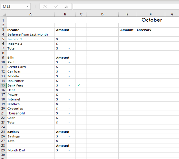
Obviously, your Bills/Savings/Income stuff will be different; this is a fairly generic example.
The important thing is to choose labels for the A column that are obvious because we will be using those in our formulas later. (Don’t worry about the B column information yet; we’ll get there; all you need are the Amount headings for each section you use). You also need an Amount and Category headings in columns. This will be where you load your daily receipts. (You don’t need the green checkmark either)
Formulas
For this sheet, you’re going to use three formulas: a Sum function, subtraction, and a SumIfs function. The Sum function will be used for our totals, the subtraction for the month end. The SumIFs function is the interesting one.
SumIFs will add up the totals of cells, but only if they meet certain criteria. In this case, we are going to set it up so that each category (B column) will add the contents of the numbers in E Column but only If they match the category criteria (F column).
We will start by setting up our basic functions in the B column. For each Total row, (B23 for example, but yours will likely be different), create a sum formula that adds up the amount in each section. For example, =Sum(B10:B22) in cell B23. In your End of Month row (B29 in the above example), we want a subtraction formula that will subtract the Total Bills and Savings from our total income. Example, =B7-B23-B27 This will give us an idea of how much money we will have at the end of the month.
Now here’s where we turn this budget into a daily. (This can also be a bit tedious, but we can make it a bit easier here and there).
For each of your actual line items, we are going to create a SumIFs formula. The trick is to ensure that you always use the same category in the formula that you will in your category column.
For example:
In cell B5, our formula will be =SumIfs(F:F,G:G,”Income1”) In cell B10, our formula will be =SumIfs(F:F,G:G,”Rent”)
We can use autofill to fill in the formulas in our income and bills area, but you will still have to change what happens between each quotes mark to fit your categories.
Testing
You should always test your formulas to make sure you haven’t missed anything. SumIfs can be easy to screw up – if you don’t write it as SumIfs (with an s!) it won’t work. You can do this by typing your rental amount in the F column and Rent in the G column beside it (under Amount and Category). As long as the rental number pops up in the right place in the B column, it worked! If not, check your function and make sure there are no errors.
You can add other bits to this sheet such as estimating how much you’ll spend in a month to make sure you come within budget, color, checkmarks, etc.
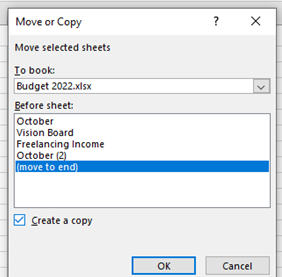
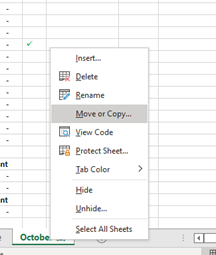
And don’t forget. To create the next month in the year, don’t redo the page! Instead, right click on the sheet tab at the bottom and click Move or Copy. Then in the dialog box, click on Create a Copy and select where you want the copy of the sheet to be placed. This way, you don’t have to redo your formulas and you just have to delete your information in the F and G column and start again each month.
Setting up a budget is daunting and many people really don’t want to think about it, but taking control of your finances helps empower your life and lets you set goals and plans more easily. Give it a try!